QuOperator in TensorCircuit#

Overview#

tensorcircuit.quantum.QuOperator, tensorcircuit.quantum.QuVector and tensorcircuit.quantum.QuAdjointVector are classes adopted from the TensorNetwork package. They behave like a matrix/vector (column or row) when interacting with other ingredients while the inner structure is maintained by the TensorNetwork for efficiency and compactness.

Typical tensor network structures for a QuOperator/QuVector correspond to Matrix Product Operators (MPO) / Matrix Product States (MPS). The former represents a matrix as: \(M_{i1,i2,...in; \; j1, j2,... jn}=\prod_k {T_k}^{i_k, j_k}\), i.e., a product of \(d\times d\) matrices \(T_k^{i_k, j_k}\), where \(d\) is known as the bond dimension. Similarly, an MPS represents a vector as: \(V_{i_1,...i_n} = \prod_k T_k^{i_k}\), where the \(T_k^{i_k}\) are, again, \(d\times d\) matrices. MPS and MPO often occur in computational quantum physics contexts, as they give compact representations for certain types of quantum states and operators.

QuOperator/QuVector objects can represent any MPO/MPS, but they can additionally express more flexible tensor network structures. Indeed, any tensor network with two sets of dangling edges of the same dimension (i.e., for each \(k\), the set \(\{T_k^{i_k,j_k}\}_{i_k,j_k}\) of matrices has \(i_k\) and \(j_k\) running over the same index set) can be treated as a QuOperator. A general QuVector is even more flexible, in that the dangling edge dimensions can be chosen freely, and thus arbitrary tensor products of vectors can be represented.

In this note, we will show how such tensor network backend matrix/vector data structure is more efficient and compact in several scenarios and how these structures integrated with quantum circuit simulation tasks seamlessly as different circuit ingredients.

Setup#

[1]:

import numpy as np
import tensornetwork as tn
import tensorcircuit as tc

print(tc.__version__)

0.0.220509

Introduction to QuOperator/QuVector#

[2]:

n1 = tc.gates.Gate(np.ones([2, 2, 2]), name="n1")
n2 = tc.gates.Gate(np.ones([2, 2, 2]), name="n2")
n3 = tc.gates.Gate(np.ones([2, 2]), name="n3")
# name is only for debug and visualization, can be omitted
n1[2] ^ n2[2]
n2[1] ^ n3[0]

# initialize a QuOperator by giving two sets of dangling edges for row and col index
matrix = tc.quantum.QuOperator(out_edges=[n1[0], n2[0]], in_edges=[n1[1], n3[1]])
tn.to_graphviz(matrix.nodes)

[2]:

../_images/whitepaper_6-4-quoperator_6_0.svg

[3]:

n4 = tc.gates.Gate(np.ones([2]), name="n4")
n5 = tc.gates.Gate(np.ones([2]), name="n5")

# initialize a QuVector by giving dangling edges
vector = tc.quantum.QuVector([n4[0], n5[0]])
tn.to_graphviz(vector.nodes)

[3]:

../_images/whitepaper_6-4-quoperator_7_0.svg

[4]:

nvector = matrix @ vector
tn.to_graphviz(nvector.nodes)
# nvector has two dangling edges

[4]:

../_images/whitepaper_6-4-quoperator_8_0.svg

[5]:

assert type(nvector) == tc.quantum.QuVector

[6]:

nvector.eval_matrix()

[6]:

array([[16.],
       [16.],
       [16.],
       [16.]])

[7]:

# or we can have more matrix/vector-like operation
(3 * nvector).eval_matrix()

[7]:

array([[48.],
       [48.],
       [48.],
       [48.]])

[8]:

matrix.partial_trace([0]).eval_matrix()

[8]:

array([[8., 8.],
       [8., 8.]])

Note how in this example, matrix is not a typical MPO but still can be expressed as QuOperator. Indeed, any tensor network with two sets of dangling edges of the same dimension can be treated as QuOperator. QuVector is even more flexible since we can treat all dangling edges as the vector dimension.

Also, note how ^ is overloaded as tn.connect to connect edges between different nodes in TensorNetwork. And indexing the node gives the edges of the node, eg. n1[0] means the first edge of node n1.

The convention to define the QuOperator is firstly giving out_edges (left index or row index of the matrix) and then giving in_edges (right index or column index of the matrix). The edges list contains edge objects from the TensorNetwork library.

Such QuOperator/QuVector abstraction support various calculations only possible on matrix/vectors, such as matmul (@), adjoint (.adjoint()), scalar multiplication (*), tensor product (|), and partial trace (.partial_trace(subsystems_to_trace_out)). To extract the matrix information of these objects, we can use .eval() or .eval_matrix(), the former keeps the shape information of the tensor network while the latter gives the matrix representation with shape rank 2.

The workflow here can also be summarized and visualized as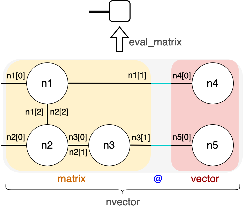

QuVector as the Input State for the Circuit#

Since QuVector behaves like a real vector with a more compact representation, we can feed the circuit input states in the form of QuVector instead of a plain numpy array vector.

[9]:

# This examples shows how we feed a |111> state into the circuit

n = 3
nodes = [tc.gates.Gate(np.array([0.0, 1.0])) for _ in range(n)]
mps = tc.quantum.QuVector([nd[0] for nd in nodes])
c = tc.Circuit(n, mps_inputs=mps)
c.x(0)
c.expectation_ps(z=[0])

[9]:

array(1.+0.j)

QuVector as the Output State of the Circuit#

The tensor network representation of the circuit can be regarded as a QuVector, namely we can manipulate the circuit as a vector before the real contraction. This is also how we do circuit composition internally.

[10]:

# Circuit composition example

n = 3
c1 = tc.Circuit(n)
c1.X(0)
c1.cnot(0, 1)
mps = c1.quvector()
c2 = tc.Circuit(n, mps_inputs=mps)
c2.X(2)
c2.X(1)
c2.cz(1, 2)
c2.expectation_ps(z=[1])
tn.to_graphviz(c2.get_quvector().nodes)

[10]:

../_images/whitepaper_6-4-quoperator_18_0.svg

[11]:

# The above is the core internal mechanism for circuit composition
# the user API is as follows

n = 3
c1 = tc.Circuit(n)
c1.X(0)
c1.cnot(0, 1)

c2 = tc.Circuit(n)
c2.X(2)
c2.X(1)
c2.cz(1, 2)
c1.append(c2)

c1.draw()

[11]:

     ┌───┐
q_0: ┤ X ├──■──────────
     └───┘┌─┴─┐┌───┐
q_1: ─────┤ X ├┤ X ├─■─
     ┌───┐└───┘└───┘ │
q_2: ┤ X ├───────────■─
     └───┘

QuOperator as Operator to be Evaluated on the Circuit#

The matrix to be evaluated over the output state of the circuit can also be represented by QuOperator, which is very powerful and efficient for some lattices model Hamiltonian.

[12]:

# Here we show the simplest model, where we measure <Z_0Z_1>

z0, z1 = tc.gates.z(), tc.gates.z()
mpo = tc.quantum.QuOperator([z0[0], z1[0]], [z0[1], z1[1]])
c = tc.Circuit(2)
c.X(0)
tc.templates.measurements.mpo_expectation(c, mpo)
# the mpo expectation API

[12]:

-1.0

QuOperator as the Quantum Gate Applied on the Circuit#

Since quantum gates are also unitary matrices, we can also use QuOperator for quantum gates. In some cases, QuOperator representation for quantum gates is much more compact, such as in multi-control gate case, where the bond dimension can be reduced to 2 for neighboring qubits.

[13]:

# The general mpo gate API is just ``Circuit.mpo()``

x0, x1 = tc.gates.Gate(np.ones([2, 2, 3]), name="x0"), tc.gates.Gate(
    np.ones([2, 2, 3]), name="x1"
)
x0[2] ^ x1[2]
mpo = tc.quantum.QuOperator([x0[0], x1[0]], [x0[1], x1[1]])
c = tc.Circuit(2)
c.mpo(0, 1, mpo=mpo)
tn.to_graphviz(c._nodes)

[13]:

../_images/whitepaper_6-4-quoperator_23_0.svg

[14]:

# the built-in multi-control gate is used as follows:

c = tc.Circuit(3)
c.multicontrol(0, 1, 2, ctrl=[0, 1], unitary=tc.gates.x())
tn.to_graphviz(c._nodes)

[14]:

../_images/whitepaper_6-4-quoperator_24_0.svg

[15]:

c.to_qir()[0]["gate"].nodes

[15]:

{Node
 (
 name : '__unnamed_node__',
 tensor :
 array([[[[0.+0.j, 1.+0.j],
          [0.+0.j, 0.+0.j]],

         [[0.+0.j, 0.+0.j],
          [1.+0.j, 0.+0.j]]],


        [[[0.+0.j, 1.+0.j],
          [0.+0.j, 0.+0.j]],

         [[0.+0.j, 0.+0.j],
          [0.+0.j, 1.+0.j]]]], dtype=complex64),
 edges :
 [
 Edge('__unnamed_node__'[2] -> '__unnamed_node__'[0] )
 ,
 Edge(Dangling Edge)[1]
 ,
 Edge(Dangling Edge)[2]
 ,
 Edge('__unnamed_node__'[3] -> '__unnamed_node__'[0] )
 ]
 ),
 Node
 (
 name : '__unnamed_node__',
 tensor :
 array([[[1.+0.j, 0.+0.j],
         [0.+0.j, 0.+0.j]],

        [[0.+0.j, 0.+0.j],
         [0.+0.j, 1.+0.j]]], dtype=complex64),
 edges :
 [
 Edge(Dangling Edge)[0]
 ,
 Edge(Dangling Edge)[1]
 ,
 Edge('__unnamed_node__'[2] -> '__unnamed_node__'[0] )
 ]
 ),
 Node
 (
 name : '__unnamed_node__',
 tensor :
 array([[[0.+0.j, 1.+0.j],
         [1.+0.j, 0.+0.j]],

        [[1.+0.j, 0.+0.j],
         [0.+0.j, 1.+0.j]]], dtype=complex64),
 edges :
 [
 Edge('__unnamed_node__'[3] -> '__unnamed_node__'[0] )
 ,
 Edge(Dangling Edge)[1]
 ,
 Edge(Dangling Edge)[2]
 ]
 )}

[16]:

c.to_qir()[0]["gate"].eval_matrix()

[16]:

array([[1.+0.j, 0.+0.j, 0.+0.j, 0.+0.j, 0.+0.j, 0.+0.j, 0.+0.j, 0.+0.j],
       [0.+0.j, 1.+0.j, 0.+0.j, 0.+0.j, 0.+0.j, 0.+0.j, 0.+0.j, 0.+0.j],
       [0.+0.j, 0.+0.j, 0.+0.j, 1.+0.j, 0.+0.j, 0.+0.j, 0.+0.j, 0.+0.j],
       [0.+0.j, 0.+0.j, 1.+0.j, 0.+0.j, 0.+0.j, 0.+0.j, 0.+0.j, 0.+0.j],
       [0.+0.j, 0.+0.j, 0.+0.j, 0.+0.j, 1.+0.j, 0.+0.j, 0.+0.j, 0.+0.j],
       [0.+0.j, 0.+0.j, 0.+0.j, 0.+0.j, 0.+0.j, 1.+0.j, 0.+0.j, 0.+0.j],
       [0.+0.j, 0.+0.j, 0.+0.j, 0.+0.j, 0.+0.j, 0.+0.j, 1.+0.j, 0.+0.j],
       [0.+0.j, 0.+0.j, 0.+0.j, 0.+0.j, 0.+0.j, 0.+0.j, 0.+0.j, 1.+0.j]],
      dtype=complex64)