Evaluation on Pauli String Sum#
Overview#
We need to evaluate the sum of many Pauli string terms on the circuit in various quantum algorithms, the ground state preparation of a Hamiltonian \(H\) in VQE is a typical example. We need to calculate the expectation value of Hamiltonian \(H\), i.e., \(\langle 0^N \vert U^{\dagger}(\theta) H U(\theta) \vert 0^N \rangle\) and update the parameters \(\theta\) in \(U(\theta)\) based on gradient descent in VQE workflow. In this tutorial, we will demonstrate five arpproaches
supported in TensorCircuit to calculate \(\langle H \rangle\):
\(\langle H \rangle = \sum_{i} \langle h_{i} \rangle\), where \(h_{i}\) are the Pauli-string operators;
Similar to 1, but we evaluate the sum of Pauli string via
vmap;\(\langle H \rangle\) where \(H\) is a sparse matrix;
\(\langle H \rangle\) where \(H\) is a dense matrix;
the expectation value of the Matrix Product Operator (MPO) for \(H\).
We consider the transverse field ising model (TFIM) as the example, which reads $ H = \sum{i} :nbsphinx-math:`sigma`{i}^{x} \sigma{i+1}^{x} - :nbsphinx-math:`sum`{i} \sigma_{i}^{z}, $ where \(\sigma_{i}^{x,z}\) are Pauli matrices of the \(i\)-th qubit.
Setup#
[1]:
import time
from functools import partial
import numpy as np
import tensorflow as tf
import tensornetwork as tn
import optax
import tensorcircuit as tc

K = tc.set_backend("tensorflow")

xx = tc.gates._xx_matrix  # xx gate matrix to be utilized
[2]:
n = 10  # The number of qubits
nlayers = 4  # The number of circuit layers
Parameterized Quantum Circuits#
[3]:
# Define the ansatz circuit to evaluate the Hamiltonian expectation
def tfim_circuit(param):
    c = tc.Circuit(n)
    for j in range(nlayers):
        for i in range(n - 1):
            c.exp1(i, i + 1, unitary=xx, theta=param[2 * j, i])
        for i in range(n):
            c.rz(i, theta=param[2 * j + 1, i])
    return c
[4]:
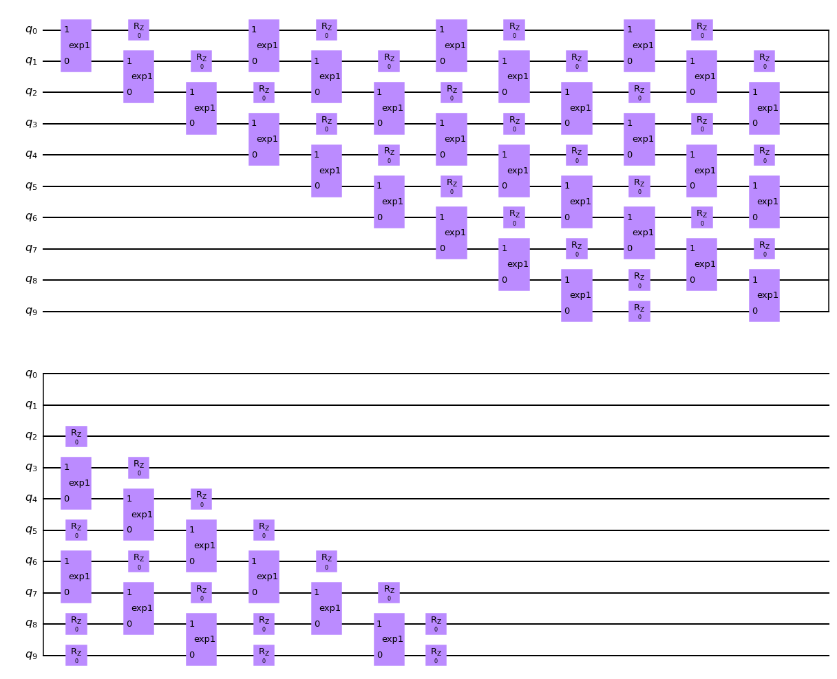
# the circuit ansatz we utilized is shown as below, the two-qubit gate is in ladder layout
tfim_circuit(K.zeros([2 * nlayers, n])).draw(output="mpl")
[4]:
Main Optimization Loop#
VQE train loop (value and grad function agnostic) is defined below.
[5]:
# We define the universal train_step function for different approaches evaluating the Pauli string sum
def train_step(vf, maxiter=400):
    param = K.implicit_randn(shape=[2 * nlayers, n], stddev=0.01)
    if K.name == "tensorflow":
        opt = K.optimizer(tf.keras.optimizers.Adam(1e-2))
    else:  # jax
        opt = K.optimizer(optax.adam(1e-2))
    vgf = tc.backend.jit(tc.backend.value_and_grad(vf))
    time0 = time.time()
    _ = vgf(param)
    time1 = time.time()
    print("staging time: ", time1 - time0)
    times = []
    for i in range(maxiter):
        time0 = time.time()
        e, grad = vgf(param)  # energy and gradients
        time1 = time.time()
        times.append(time1 - time0)
        param = opt.update(grad, param)
        if i % 200 == 0:
            print(e)
    print("running time: ", np.mean(times))
    return e
1. Pauli-string Operators Sum#
[6]:
# Sum the Pauli string expectation in a plain way
def tfim_energy(c, j=1.0, h=-1.0):
    e = 0.0
    n = c._nqubits
    for i in range(n):
        e += h * c.expectation_ps(z=[i])  # <Z_i>
    for i in range(n - 1):  # OBC
        e += j * c.expectation_ps(x=[i, i + 1])  # <X_iX_{i+1}>
    return K.real(e)
[7]:
def vqe_tfim_v1(param):
    c = tfim_circuit(param)
    e = tfim_energy(c)
    return e
[8]:
train_step(vqe_tfim_v1)
staging time:  29.903974294662476
tf.Tensor(-9.9926815, shape=(), dtype=float32)
tf.Tensor(-11.69182, shape=(), dtype=float32)
running time:  0.004392582178115845
[8]:
<tf.Tensor: shape=(), dtype=float32, numpy=-11.658401>
2. Vmap the Pauli-string Operators Sum#
A string of Pauli operators acting on \(n\) qubits can be represented as a length \(n\) vector \(v\in\{0,1,2,3\}^n\), where the value of \(v_i = j\) corresponds to \(\sigma_i^j\), i.e. Pauli operator \(\sigma^j\) acting on qubit \(i\) (with \(\sigma^0 = I, \sigma^1 = X, \sigma^2 = Y, \sigma^3 = Z\)). For example, in this notation, if \(n=3\) the term \(X_1 X_2\) corresponds to \(v = [0,1,1]\). We refer to such a vector representation of a Pauli string
as a structure, and a list of structures, one for each Pauli string term in the Hamiltonian, is used as the input to compute sums of expectation values in a number of ways.
If each structure has an associated weight, e.g. the term \(X_i X_{i+1}\) has weight \(J_i\) in TFIM Hamiltonian, then we define a corresponding tensor of weights.
[9]:
def measurement(s, structure):
    c = tc.Circuit(n, inputs=s)
    return tc.templates.measurements.parameterized_measurements(
        c, structure, onehot=True
    )


measurement = K.jit(K.vmap(measurement, vectorized_argnums=1))

structures = []
for i in range(n - 1):
    s = [0 for _ in range(n)]
    s[i] = 1
    s[i + 1] = 1
    structures.append(s)
for i in range(n):
    s = [0 for _ in range(n)]
    s[i] = 3
    structures.append(s)

structures = tc.array_to_tensor(structures)
weights = tc.array_to_tensor(
    np.array([1.0 for _ in range(n - 1)] + [-1.0 for _ in range(n)])
)

print(K.numpy(structures))
print(K.numpy(weights))


def vqe_tfim_v2(param):
    c = tfim_circuit(param)
    s = c.state()
    ms = measurement(s, structures)
    return K.sum(ms * K.real(weights))
[[1.+0.j 1.+0.j 0.+0.j 0.+0.j 0.+0.j 0.+0.j 0.+0.j 0.+0.j 0.+0.j 0.+0.j]
 [0.+0.j 1.+0.j 1.+0.j 0.+0.j 0.+0.j 0.+0.j 0.+0.j 0.+0.j 0.+0.j 0.+0.j]
 [0.+0.j 0.+0.j 1.+0.j 1.+0.j 0.+0.j 0.+0.j 0.+0.j 0.+0.j 0.+0.j 0.+0.j]
 [0.+0.j 0.+0.j 0.+0.j 1.+0.j 1.+0.j 0.+0.j 0.+0.j 0.+0.j 0.+0.j 0.+0.j]
 [0.+0.j 0.+0.j 0.+0.j 0.+0.j 1.+0.j 1.+0.j 0.+0.j 0.+0.j 0.+0.j 0.+0.j]
 [0.+0.j 0.+0.j 0.+0.j 0.+0.j 0.+0.j 1.+0.j 1.+0.j 0.+0.j 0.+0.j 0.+0.j]
 [0.+0.j 0.+0.j 0.+0.j 0.+0.j 0.+0.j 0.+0.j 1.+0.j 1.+0.j 0.+0.j 0.+0.j]
 [0.+0.j 0.+0.j 0.+0.j 0.+0.j 0.+0.j 0.+0.j 0.+0.j 1.+0.j 1.+0.j 0.+0.j]
 [0.+0.j 0.+0.j 0.+0.j 0.+0.j 0.+0.j 0.+0.j 0.+0.j 0.+0.j 1.+0.j 1.+0.j]
 [3.+0.j 0.+0.j 0.+0.j 0.+0.j 0.+0.j 0.+0.j 0.+0.j 0.+0.j 0.+0.j 0.+0.j]
 [0.+0.j 3.+0.j 0.+0.j 0.+0.j 0.+0.j 0.+0.j 0.+0.j 0.+0.j 0.+0.j 0.+0.j]
 [0.+0.j 0.+0.j 3.+0.j 0.+0.j 0.+0.j 0.+0.j 0.+0.j 0.+0.j 0.+0.j 0.+0.j]
 [0.+0.j 0.+0.j 0.+0.j 3.+0.j 0.+0.j 0.+0.j 0.+0.j 0.+0.j 0.+0.j 0.+0.j]
 [0.+0.j 0.+0.j 0.+0.j 0.+0.j 3.+0.j 0.+0.j 0.+0.j 0.+0.j 0.+0.j 0.+0.j]
 [0.+0.j 0.+0.j 0.+0.j 0.+0.j 0.+0.j 3.+0.j 0.+0.j 0.+0.j 0.+0.j 0.+0.j]
 [0.+0.j 0.+0.j 0.+0.j 0.+0.j 0.+0.j 0.+0.j 3.+0.j 0.+0.j 0.+0.j 0.+0.j]
 [0.+0.j 0.+0.j 0.+0.j 0.+0.j 0.+0.j 0.+0.j 0.+0.j 3.+0.j 0.+0.j 0.+0.j]
 [0.+0.j 0.+0.j 0.+0.j 0.+0.j 0.+0.j 0.+0.j 0.+0.j 0.+0.j 3.+0.j 0.+0.j]
 [0.+0.j 0.+0.j 0.+0.j 0.+0.j 0.+0.j 0.+0.j 0.+0.j 0.+0.j 0.+0.j 3.+0.j]]
[ 1.+0.j  1.+0.j  1.+0.j  1.+0.j  1.+0.j  1.+0.j  1.+0.j  1.+0.j  1.+0.j
 -1.+0.j -1.+0.j -1.+0.j -1.+0.j -1.+0.j -1.+0.j -1.+0.j -1.+0.j -1.+0.j
 -1.+0.j]
[10]:
train_step(vqe_tfim_v2)
staging time:  18.228847980499268
tf.Tensor(-9.991278, shape=(), dtype=float32)
tf.Tensor(-11.868717, shape=(), dtype=float32)
running time:  0.00716902494430542
[10]:
<tf.Tensor: shape=(), dtype=float32, numpy=-11.842572>
3. Sparse Matrix#
The significant computational advantage in terms of space and time can be obtained if the Hamiltonian is sparse, in which case a sparse representation of the operator is preferable. This can be provided in a backend agnostic way by converting from a list of Pauli structures in a two-stage process. First, we convert it to a sparse numpy matrix in COO (COOrdinate) format, and then we convert it to coo sparse tensor on a given ML backend.
[11]:
def vqe_tfim_template(param, op):
    c = tfim_circuit(param)
    e = tc.templates.measurements.operator_expectation(
        c, op
    )  # in operator_expectation, the "hamiltonian" can be a sparse matrix, dense matrix or mpo
    return e
[12]:
# We first generate the Hamiltonian matrix as follows

hamiltonian_sparse_numpy = tc.quantum.PauliStringSum2COO_numpy(structures, weights)
hamiltonian_sparse_numpy
[12]:
<1024x1024 sparse matrix of type '<class 'numpy.complex64'>'
        with 9988 stored elements in COOrdinate format>
[13]:
hamiltonian_sparse = K.coo_sparse_matrix(
    np.transpose(
        np.stack([hamiltonian_sparse_numpy.row, hamiltonian_sparse_numpy.col])
    ),
    hamiltonian_sparse_numpy.data,
    shape=(2**n, 2**n),
)
[14]:
vqe_tfim_v3 = partial(vqe_tfim_template, op=hamiltonian_sparse)
[15]:
train_step(vqe_tfim_v3)
staging time:  13.532029867172241
tf.Tensor(-9.976083, shape=(), dtype=float32)
tf.Tensor(-11.907323, shape=(), dtype=float32)
running time:  0.002562386989593506
[15]:
<tf.Tensor: shape=(), dtype=float32, numpy=-11.875302>
4. Dense Matrix#
[16]:
hamiltonian_dense = K.to_dense(hamiltonian_sparse)
[17]:
vqe_tfim_v4 = partial(vqe_tfim_template, op=hamiltonian_dense)
[18]:
train_step(vqe_tfim_v4)
staging time:  15.174713850021362
tf.Tensor(-9.981074, shape=(), dtype=float32)
tf.Tensor(-11.836525, shape=(), dtype=float32)
running time:  0.0039513856172561646
[18]:
<tf.Tensor: shape=(), dtype=float32, numpy=-11.799629>
5. MPO#
The TFIM Hamiltonian, as a short-ranged spin Hamiltonian, admits an efficient Matrix Product Operator representation. Again this is a two-stage process using TensorCircuit. We first convert the Hamiltonian into an MPO representation via the TensorNetwork or Quimb package.
[19]:
# generate the corresponding MPO by converting the MPO in tensornetwork package

Jx = np.array([1.0 for _ in range(n - 1)])  # strength of xx interaction (OBC)
Bz = np.array([1.0 for _ in range(n)])  # strength of transverse field
# Note the convention for the sign of Bz
hamiltonian_mpo = tn.matrixproductstates.mpo.FiniteTFI(
    Jx, Bz, dtype=np.complex64
)  # matrix product operator in TensorNetwork
hamiltonian_mpo = tc.quantum.tn2qop(hamiltonian_mpo)  # QuOperator in TensorCircuit
[20]:
vqe_tfim_v5 = partial(vqe_tfim_template, op=hamiltonian_mpo)
[21]:
train_step(vqe_tfim_v5)
staging time:  26.719671964645386
tf.Tensor(-9.985788, shape=(), dtype=float32)
tf.Tensor(-11.857734, shape=(), dtype=float32)
running time:  0.00492021381855011
[21]:
<tf.Tensor: shape=(), dtype=float32, numpy=-11.828297>