Classical Shadows in Pauli Basis#
Overview#
Classical shadows formalism is an efficient method to estimate multiple observables. In this tutorial, we will show how to use the shadows module in TensorCircuit to implement classic shadows in Pauli basis.
Let’s first briefly review the classical shadows in Pauli basis. For an \(n\)-qubit quantum state \(\rho\), we randomly perform Pauli projection measurement on each qubit and obtain a snapshot like \(\{1,-1,-1,1,\cdots,1,-1\}\). This process is equivalent to apply a random unitary \(U_i\) to \(\rho\) and measure in computational basis to obtain \(|b_i\rangle=|s_{i1}\cdots s_{in}\rangle,\ s_{ij}\in\{0,1\}\):
where \(U_i=\bigotimes_{j=1}^{n}u_{ij}\), \(u_{ij}\in\{H, HS^{\dagger}, \mathbb{I}\}\) correspond to the projection measurements of Pauli \(X\), \(Y\), \(Z\) respectively. Then we reverse the operation to get the equivalent measurement result on \(\rho\):
Moreover, we perform \(N\) random measurements and view their average as a quantum channel:
we can invert the channel to get the approximation of \(\rho\):
We call each \(\rho_i=\mathcal{M}^{-1}(U_i^{\dagger}|b_i\rangle\langle b_i|U_i)\) a shadow snapshot state and their ensemble \(S(\rho;N)=\{\rho_i|i=1,\cdots,N\}\) classical shadows.
In Pauli basis, we have a simple expression of \(\mathcal{M}^{-1}\):
For an observable Pauli string \(O=\bigotimes_{j=1}^{n}P_j,\ P_j\in\{\mathbb{I}, X, Y, Z\}\), we can directly use \(\rho\) to calculate \(\langle O\rangle=\text{Tr}(O\rho)\). In practice, we will divide the classical shadows into \(K\) parts to calculate the expectation values independently and take the median to avoid the influence of outliers:
where
Setup#
[13]:
import tensorcircuit as tc
from tensorcircuit import shadows
import numpy as np
from functools import partial
import time
import matplotlib.pyplot as plt

tc.set_backend("jax")
tc.set_dtype("complex128")
[13]:
('complex128', 'float64')
Construct the Classical Shadow Snapshots#
We first set the number of qubits \(n\) and the number of repeated measurements \(r\) on each Pauli string. Then from the target observable Pauli strings \(\{O_i|i=1,\cdots,M\}\) (0, 1, 2, and 3 correspond to \(\mathbb{I}\), \(X\), \(Y\), and \(Z\), respectively), the error \(\epsilon\) and the rate of failure \(\delta\), we can use shadow_bound function to get the total number of snapshots \(N\) and the number of equal parts \(K\) to split the
shadow snapshot states to compute the median of means:
where \(k_i\) is the number of nontrivial Pauli matrices in \(O_i\). Please refer to the Theorem S1 and Lemma S3 in Huang, Kueng and Preskill (2020) for the details of proof. It should be noted that shadow_bound has a certain degree of overestimation of \(N\), and so many measurements are not really needed in practice. Moreover, shadow_bound is not jitable and no need to jit.
[14]:
n, r = 8, 5
ps = [
    [1, 0, 0, 0, 0, 0, 0, 2],
    [0, 3, 0, 0, 0, 0, 1, 0],
    [0, 0, 2, 0, 0, 3, 0, 0],
    [0, 0, 0, 1, 2, 0, 0, 0],
    [0, 0, 0, 3, 1, 0, 0, 0],
    [0, 0, 0, 0, 0, 3, 0, 0],
    [0, 0, 0, 0, 0, 0, 2, 0],
    [3, 0, 0, 0, 0, 0, 0, 1],
    [0, 2, 0, 0, 0, 0, 3, 0],
    [0, 0, 1, 0, 0, 2, 0, 0],
]

epsilon, delta = 0.1, 0.01
N, K = shadows.shadow_bound(ps, epsilon, delta)
nps = N // r  # number of random selected Pauli strings
print(f"N: {N}\tK: {K}\tnumber of Pauli strings: {nps}")
N: 489600 K: 16 number of Pauli strings: 97920
Then we use random quantum circuit to generate an entangled state.
[15]:
nlayers = 10
thetas = 2 * np.random.rand(nlayers, n) - 1

c = tc.Circuit(n)
for i in range(n):
    c.H(i)
for i in range(nlayers):
    for j in range(n):
        c.cnot(j, (j + 1) % n)
    for j in range(n):
        c.rz(j, theta=thetas[i, j] * np.pi)

psi = c.state()
We randomly generate Pauli strings. Since the function after just-in-time (jit) compilation does not support random sampling, we need to generate all random states in advance, that is, variable status.
[16]:
pauli_strings = tc.backend.convert_to_tensor(np.random.randint(1, 4, size=(nps, n)))
status = tc.backend.convert_to_tensor(np.random.rand(nps, r))
If measurement_only=True (default False), the outputs of shadow_snapshots are snapshot bit strings \(\{b_i=s_{i1}\cdots s_{in}\ |i=1,\cdots,N,\ s_{ij}\in\{0,1\}\}\), otherwise the outputs are snapshot states \(\{u_{ij}^{\dagger}|s_{ij}\rangle\langle s_{ij}| u_{ij}\ |i=1,\cdots,N,\ j=1,\cdots,n\}\). If you only need to generate one batch of snapshots or generate multiple batches of snapshots with different nps or r, jit cannot provide speedup. Jit will only accelerate
when the same shape of snapshots are generated multiple times.
[17]:
@partial(tc.backend.jit, static_argnums=(3,))
def shadow_ss(psi, pauli_strings, status, measurement_only=False):
    return shadows.shadow_snapshots(
        psi, pauli_strings, status, measurement_only=measurement_only
    )


ss_states = shadow_ss(psi, pauli_strings, status)  # jit is not necessary here
print("shape of snapshot states:", ss_states.shape)
shape of snapshot states: (97920, 5, 8, 2, 2)
Estimate the Expectation Values of Observables#
Since the operation of taking the median is not jitable, the outputs of expectation_ps_shadows have \(K\) values, and we need to take the median of them.
[18]:
def shadow_expec(snapshots_states, ob):
    return shadows.expectation_ps_shadow(snapshots_states, ps=ob, k=K)


sejit = tc.backend.jit(shadow_expec)
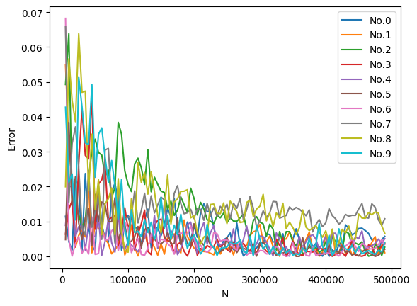
It can be seen from the running time that every time the number of Pauli strings changes, shadow_expec will be recompiled, but for the same number of Pauli strings but different observables, shadow_expec will only be compiled once. In the end, the absolute errors given by classical shadows are much smaller than the \(\epsilon=0.1\) we set, so shadow_bound gives a very loose upper bound.
[19]:
bz = 1000

exact = []
for ob in ps:
    exact.append(tc.backend.real(c.expectation_ps(ps=ob)))
exact = np.asarray(exact)[:, None]

bzs, res = [], []
for i in range(bz, nps + bz, bz):
    res.append([])
    ss_states_batch = ss_states[:i]
    bzs.append(ss_states_batch.shape[0])
    t0 = time.time()
    for j, ob in enumerate(ps):
        expcs = sejit(ss_states_batch, ob)
        res[-1].append(np.median(expcs))
        t = time.time()
        if i == bz or i % (bz * 10) == 0 or i >= nps:
            print(
                f"observable: No.{j}\tnumber of Pauli strings: {bzs[-1]}\ttime: {t - t0}"
            )
        t0 = t
res = np.asarray(res).T
bzs = np.asarray(bzs) * r

error = np.abs(res - exact)
plt.figure()
plt.xlabel("N")
plt.ylabel("Error")
for i, y in enumerate(error):
    plt.plot(bzs, y, label=f"No.{i}")
plt.legend()
plt.show()
observable: No.0        number of Pauli strings: 1000   time: 0.9454922676086426
observable: No.1        number of Pauli strings: 1000   time: 0.001840353012084961
observable: No.2        number of Pauli strings: 1000   time: 0.0014374256134033203
observable: No.3        number of Pauli strings: 1000   time: 0.0013763904571533203
observable: No.4        number of Pauli strings: 1000   time: 0.0013554096221923828
observable: No.5        number of Pauli strings: 1000   time: 0.0013613700866699219
observable: No.6        number of Pauli strings: 1000   time: 0.0013325214385986328
observable: No.7        number of Pauli strings: 1000   time: 0.0013136863708496094
observable: No.8        number of Pauli strings: 1000   time: 0.0013325214385986328
observable: No.9        number of Pauli strings: 1000   time: 0.0013117790222167969
observable: No.0        number of Pauli strings: 10000  time: 0.9969091415405273
observable: No.1        number of Pauli strings: 10000  time: 0.012966394424438477
observable: No.2        number of Pauli strings: 10000  time: 0.012765884399414062
observable: No.3        number of Pauli strings: 10000  time: 0.012974739074707031
observable: No.4        number of Pauli strings: 10000  time: 0.012665033340454102
observable: No.5        number of Pauli strings: 10000  time: 0.012889623641967773
observable: No.6        number of Pauli strings: 10000  time: 0.013180255889892578
observable: No.7        number of Pauli strings: 10000  time: 0.012682914733886719
observable: No.8        number of Pauli strings: 10000  time: 0.012678146362304688
observable: No.9        number of Pauli strings: 10000  time: 0.012636423110961914
observable: No.0        number of Pauli strings: 20000  time: 1.015674352645874
observable: No.1        number of Pauli strings: 20000  time: 0.025749921798706055
observable: No.2        number of Pauli strings: 20000  time: 0.02578139305114746
observable: No.3        number of Pauli strings: 20000  time: 0.02524733543395996
observable: No.4        number of Pauli strings: 20000  time: 0.025956153869628906
observable: No.5        number of Pauli strings: 20000  time: 0.02669525146484375
observable: No.6        number of Pauli strings: 20000  time: 0.026634931564331055
observable: No.7        number of Pauli strings: 20000  time: 0.026463985443115234
observable: No.8        number of Pauli strings: 20000  time: 0.0273745059967041
observable: No.9        number of Pauli strings: 20000  time: 0.026821374893188477
observable: No.0        number of Pauli strings: 30000  time: 1.0086262226104736
observable: No.1        number of Pauli strings: 30000  time: 0.03922295570373535
observable: No.2        number of Pauli strings: 30000  time: 0.038678884506225586
observable: No.3        number of Pauli strings: 30000  time: 0.03868269920349121
observable: No.4        number of Pauli strings: 30000  time: 0.04024958610534668
observable: No.5        number of Pauli strings: 30000  time: 0.03927755355834961
observable: No.6        number of Pauli strings: 30000  time: 0.039815664291381836
observable: No.7        number of Pauli strings: 30000  time: 0.04002213478088379
observable: No.8        number of Pauli strings: 30000  time: 0.03934764862060547
observable: No.9        number of Pauli strings: 30000  time: 0.04060721397399902
observable: No.0        number of Pauli strings: 40000  time: 1.2912404537200928
observable: No.1        number of Pauli strings: 40000  time: 0.05326724052429199
observable: No.2        number of Pauli strings: 40000  time: 0.05272030830383301
observable: No.3        number of Pauli strings: 40000  time: 0.054486989974975586
observable: No.4        number of Pauli strings: 40000  time: 0.0538792610168457
observable: No.5        number of Pauli strings: 40000  time: 0.05555129051208496
observable: No.6        number of Pauli strings: 40000  time: 0.05361533164978027
observable: No.7        number of Pauli strings: 40000  time: 0.05325675010681152
observable: No.8        number of Pauli strings: 40000  time: 0.05487465858459473
observable: No.9        number of Pauli strings: 40000  time: 0.05441641807556152
observable: No.0        number of Pauli strings: 50000  time: 0.999931812286377
observable: No.1        number of Pauli strings: 50000  time: 0.06137228012084961
observable: No.2        number of Pauli strings: 50000  time: 0.06159329414367676
observable: No.3        number of Pauli strings: 50000  time: 0.06138134002685547
observable: No.4        number of Pauli strings: 50000  time: 0.060491085052490234
observable: No.5        number of Pauli strings: 50000  time: 0.06045842170715332
observable: No.6        number of Pauli strings: 50000  time: 0.0629739761352539
observable: No.7        number of Pauli strings: 50000  time: 0.06146860122680664
observable: No.8        number of Pauli strings: 50000  time: 0.061437129974365234
observable: No.9        number of Pauli strings: 50000  time: 0.061475515365600586
observable: No.0        number of Pauli strings: 60000  time: 1.03033447265625
observable: No.1        number of Pauli strings: 60000  time: 0.06811189651489258
observable: No.2        number of Pauli strings: 60000  time: 0.06913161277770996
observable: No.3        number of Pauli strings: 60000  time: 0.06945395469665527
observable: No.4        number of Pauli strings: 60000  time: 0.06843304634094238
observable: No.5        number of Pauli strings: 60000  time: 0.06950116157531738
observable: No.6        number of Pauli strings: 60000  time: 0.07009696960449219
observable: No.7        number of Pauli strings: 60000  time: 0.06856656074523926
observable: No.8        number of Pauli strings: 60000  time: 0.06969141960144043
observable: No.9        number of Pauli strings: 60000  time: 0.0678703784942627
observable: No.0        number of Pauli strings: 70000  time: 1.0191996097564697
observable: No.1        number of Pauli strings: 70000  time: 0.07705307006835938
observable: No.2        number of Pauli strings: 70000  time: 0.07620859146118164
observable: No.3        number of Pauli strings: 70000  time: 0.07670450210571289
observable: No.4        number of Pauli strings: 70000  time: 0.0766746997833252
observable: No.5        number of Pauli strings: 70000  time: 0.07552027702331543
observable: No.6        number of Pauli strings: 70000  time: 0.07716488838195801
observable: No.7        number of Pauli strings: 70000  time: 0.07647228240966797
observable: No.8        number of Pauli strings: 70000  time: 0.07623863220214844
observable: No.9        number of Pauli strings: 70000  time: 0.07545590400695801
observable: No.0        number of Pauli strings: 80000  time: 1.0341267585754395
observable: No.1        number of Pauli strings: 80000  time: 0.08658909797668457
observable: No.2        number of Pauli strings: 80000  time: 0.08614206314086914
observable: No.3        number of Pauli strings: 80000  time: 0.0857245922088623
observable: No.4        number of Pauli strings: 80000  time: 0.08441877365112305
observable: No.5        number of Pauli strings: 80000  time: 0.08495783805847168
observable: No.6        number of Pauli strings: 80000  time: 0.08582544326782227
observable: No.7        number of Pauli strings: 80000  time: 0.0861966609954834
observable: No.8        number of Pauli strings: 80000  time: 0.08437252044677734
observable: No.9        number of Pauli strings: 80000  time: 0.0852508544921875
observable: No.0        number of Pauli strings: 90000  time: 1.031904697418213
observable: No.1        number of Pauli strings: 90000  time: 0.09243512153625488
observable: No.2        number of Pauli strings: 90000  time: 0.09180665016174316
observable: No.3        number of Pauli strings: 90000  time: 0.09398865699768066
observable: No.4        number of Pauli strings: 90000  time: 0.09126615524291992
observable: No.5        number of Pauli strings: 90000  time: 0.09299516677856445
observable: No.6        number of Pauli strings: 90000  time: 0.09152960777282715
observable: No.7        number of Pauli strings: 90000  time: 0.09381914138793945
observable: No.8        number of Pauli strings: 90000  time: 0.09076142311096191
observable: No.9        number of Pauli strings: 90000  time: 0.08988714218139648
observable: No.0        number of Pauli strings: 97920  time: 1.050750494003296
observable: No.1        number of Pauli strings: 97920  time: 0.09993815422058105
observable: No.2        number of Pauli strings: 97920  time: 0.10038924217224121
observable: No.3        number of Pauli strings: 97920  time: 0.09895133972167969
observable: No.4        number of Pauli strings: 97920  time: 0.09973955154418945
observable: No.5        number of Pauli strings: 97920  time: 0.10170507431030273
observable: No.6        number of Pauli strings: 97920  time: 0.09864187240600586
observable: No.7        number of Pauli strings: 97920  time: 0.09945058822631836
observable: No.8        number of Pauli strings: 97920  time: 0.09991574287414551
observable: No.9        number of Pauli strings: 97920  time: 0.09802794456481934
Estimate the Entanglement Entropy#
We can also use classical shadows to calculate entanglement entropy. entropy_shadow first reconstructs the reduced density matrix, then solves the eigenvalues and finally calculates the entanglement entropy from non-negative eigenvalues. Since the time and space complexity of reconstructing the density matrix is exponential with respect to the system size, this method is only efficient when the reduced system size is constant. entropy_shadow is jitable, but it will only accelerate when
the reduced sub systems have the same shape.
[20]:
subs = [
    [1, 4],
    [2, 7],
    [3, 6],
    [0, 5],
    [7, 0],
    [1, 4, 7],
    [0, 3, 6],
    [5, 4, 2],
    [7, 2, 5],
    [0, 1, 2],
]


@tc.backend.jit
def shadow_ent(snapshots_states, sub, alpha=2):
    return shadows.entropy_shadow(snapshots_states, sub=sub, alpha=alpha)


for sub in subs:
    exact_rdm = tc.quantum.reduced_density_matrix(
        psi, cut=[i for i in range(n) if i not in sub]
    )
    exact_ent = tc.quantum.renyi_entropy(exact_rdm, k=2)

    t0 = time.time()
    ent = shadow_ent(ss_states, sub)
    t = time.time()
    print(f"sub: {sub}\ttime: {t - t0}\texact: {exact_ent}\tshadow entropy: {ent}")
sub: [1, 4]     time: 0.1788625717163086        exact: 1.3222456063743848       shadow entropy: 1.323659494989336
sub: [2, 7]     time: 0.03922629356384277       exact: 1.313932933107046        shadow entropy: 1.315937416629094
sub: [3, 6]     time: 0.03881263732910156       exact: 1.342032043092265        shadow entropy: 1.3427963599754822
sub: [0, 5]     time: 0.03893852233886719       exact: 1.3458706554536102       shadow entropy: 1.346507278883028
sub: [7, 0]     time: 0.039243221282958984      exact: 1.3496695271830874       shadow entropy: 1.3504498597279848
sub: [1, 4, 7]  time: 0.2567908763885498        exact: 1.8741003653918944       shadow entropy: 1.8777698830270055
sub: [0, 3, 6]  time: 0.11173439025878906       exact: 1.8633273061204374       shadow entropy: 1.8638162138941512
sub: [5, 4, 2]  time: 0.11144137382507324       exact: 1.908653965480665        shadow entropy: 1.9084333256925539
sub: [7, 2, 5]  time: 0.1119997501373291        exact: 1.8916979397866593       shadow entropy: 1.88828077605345
sub: [0, 1, 2]  time: 0.11184382438659668       exact: 1.8717789129825904       shadow entropy: 1.8724197548909916
On the other hand, for the second order Renyi entropy, we have another method to calculate it in polynomial time by random measurements:
where \(A\) is the \(k\)-d reduced system, \(H(b,b')\) is the Hamming distance between \(b\) and \(b'\), \(P(b)\) is the probability for measuring \(\rho_A\) and obtaining the outcomes \(b\) thus we need a larger \(r\) to obtain a good enough priori probability, and the overline means the average on all random selected Pauli strings. Please refer to Brydges, et al. (2019) for more details. We can
use renyi_entropy_2 to implement this method, but it is not jitable because we need to build the dictionary based on the bit strings obtained by measurements, which is a dynamical process. Compared with entropy_shadow, it cannot filter out non-negative eigenvalues, so the accuracy is slightly worse.
[21]:
nps, r = 1000, 500

pauli_strings = tc.backend.convert_to_tensor(np.random.randint(1, 4, size=(nps, n)))
status = tc.backend.convert_to_tensor(np.random.rand(nps, r))

snapshots = shadows.shadow_snapshots(psi, pauli_strings, status, measurement_only=True)

t0 = time.time()
for sub in subs:
    ent2 = shadows.renyi_entropy_2(snapshots, sub)

    t = time.time()
    print(f"sub: {sub}\ttime: {t - t0}\tshadow entropy 2: {ent2}")
    t0 = t
sub: [1, 4]     time: 3.794407606124878 shadow entropy 2: 1.2866729353788704
sub: [2, 7]     time: 3.796651840209961 shadow entropy 2: 1.2875279355654872
sub: [3, 6]     time: 3.760688066482544 shadow entropy 2: 1.314993963087972
sub: [0, 5]     time: 3.765700101852417 shadow entropy 2: 1.317198599992926
sub: [7, 0]     time: 3.784120559692383 shadow entropy 2: 1.3218300427352758
sub: [1, 4, 7]  time: 3.859661817550659 shadow entropy 2: 1.7701671972428563
sub: [0, 3, 6]  time: 3.874009132385254 shadow entropy 2: 1.7684695179560657
sub: [5, 4, 2]  time: 3.831859827041626 shadow entropy 2: 1.8037352454314826
sub: [7, 2, 5]  time: 3.824885368347168 shadow entropy 2: 1.8006117836020135
sub: [0, 1, 2]  time: 3.8377578258514404        shadow entropy 2: 1.782393800345501
Reconstruct the Density Matrix#
We can use global_shadow_state, global_shadow_state1 or global_shadow_state2 to reconstruct the density matrix. These three functions use different methods, but the results are exactly the same. All functions are jitable, but since we only use each of them once here, they are not wrapped. In terms of implementation details, global_shadow_state uses kron and is recommended, the other two use einsum.
[22]:
n, nps, r = 2, 10000, 5

c = tc.Circuit(n)
c.H(0)
c.cnot(0, 1)

psi = c.state()
bell_state = psi[:, None] @ psi[None, :]

pauli_strings = tc.backend.convert_to_tensor(np.random.randint(1, 4, size=(nps, n)))
status = tc.backend.convert_to_tensor(np.random.rand(nps, r))
lss_states = shadows.shadow_snapshots(psi, pauli_strings, status)
sdw_state = shadows.global_shadow_state(lss_states)
sdw_state1 = shadows.global_shadow_state1(lss_states)
sdw_state2 = shadows.global_shadow_state2(lss_states)

print("exact:\n", bell_state)
print(f"\nshadow state: error: {np.linalg.norm(bell_state - sdw_state)}\n", sdw_state)
print(
    f"\nshadow state 1: error: {np.linalg.norm(bell_state - sdw_state)}\n", sdw_state1
)
print(
    f"\nshadow state 2: error: {np.linalg.norm(bell_state - sdw_state)}\n", sdw_state2
)
exact:
 [[0.5+0.j 0. +0.j 0. +0.j 0.5+0.j]
 [0. +0.j 0. +0.j 0. +0.j 0. +0.j]
 [0. +0.j 0. +0.j 0. +0.j 0. +0.j]
 [0.5+0.j 0. +0.j 0. +0.j 0.5+0.j]]

shadow state: error: 0.02441655995426051
 [[ 0.49141+0.j       0.00159+0.00219j  0.00378+0.00306j  0.5004 +0.0081j ]
 [ 0.00159-0.00219j  0.0019 +0.j      -0.00855+0.00297j -0.00567-0.00126j]
 [ 0.00378-0.00306j -0.00855-0.00297j  0.00805+0.j      -0.00273-0.00249j]
 [ 0.5004 -0.0081j  -0.00567+0.00126j -0.00273+0.00249j  0.49864+0.j     ]]

shadow state 1: error: 0.02441655995426051
 [[ 0.49141+0.j       0.00159+0.00219j  0.00378+0.00306j  0.5004 +0.0081j ]
 [ 0.00159-0.00219j  0.0019 +0.j      -0.00855+0.00297j -0.00567-0.00126j]
 [ 0.00378-0.00306j -0.00855-0.00297j  0.00805+0.j      -0.00273-0.00249j]
 [ 0.5004 -0.0081j  -0.00567+0.00126j -0.00273+0.00249j  0.49864+0.j     ]]

shadow state 2: error: 0.02441655995426051
 [[ 0.49141+0.j       0.00159+0.00219j  0.00378+0.00306j  0.5004 +0.0081j ]
 [ 0.00159-0.00219j  0.0019 +0.j      -0.00855+0.00297j -0.00567-0.00126j]
 [ 0.00378-0.00306j -0.00855-0.00297j  0.00805+0.j      -0.00273-0.00249j]
 [ 0.5004 -0.0081j  -0.00567+0.00126j -0.00273+0.00249j  0.49864+0.j     ]]
[23]:
tc.about()
OS info: Linux-5.4.119-1-tlinux4-0010.2-x86_64-with-glibc2.28
Python version: 3.10.11
Numpy version: 1.23.5
Scipy version: 1.11.0
Pandas version: 2.0.2
TensorNetwork version: 0.4.6
Cotengra version: 0.2.1.dev15+g120379e
TensorFlow version: 2.12.0
TensorFlow GPU: []
TensorFlow CUDA infos: {'cpu_compiler': '/dt9/usr/bin/gcc', 'cuda_compute_capabilities': ['sm_35', 'sm_50', 'sm_60', 'sm_70', 'sm_75', 'compute_80'], 'cuda_version': '11.8', 'cudnn_version': '8', 'is_cuda_build': True, 'is_rocm_build': False, 'is_tensorrt_build': True}
Jax version: 0.4.13
Jax installation doesn't support GPU
JaxLib version: 0.4.13
PyTorch version: 2.0.1
PyTorch GPU support: False
PyTorch GPUs: []
Cupy is not installed
Qiskit version: 0.24.1
Cirq version: 1.1.0
TensorCircuit version 0.10.0