Quantum Machine Learning for Classification Task#
Demonstrations on some common setups and techniques
Overview#
We use the fashion-MNIST dataset to set up a binary classification task, we will try different encoding schemes for the inputs and apply possible classical post-processing on the quantum outputs to enhance the classification accuracy. In this tutorial, we stick to the TensorFlow backend and try to consistently use the Keras interface provided by tensorcircuit for quantum functions, where we can magically turn a quantum function into a Keras layer.
[1]:
from matplotlib import pyplot as plt
from sklearn.decomposition import PCA
import tensorflow as tf
import tensorcircuit as tc

K = tc.set_backend("tensorflow")
Dataset and Pre-processing#
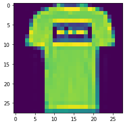
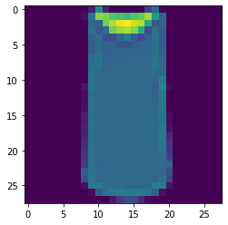
We first load the fashion-mnist dataset and differentiation between T-shirt (0) and Trouser (1).
[2]:
(x_train, y_train), (x_test, y_test) = tc.templates.dataset.mnist_pair_data(
    0, 1, loader=tf.keras.datasets.fashion_mnist
)
[3]:
x_train.shape, y_train.shape, x_test.shape, y_test.shape
[3]:
((12000, 28, 28, 1), (12000,), (2000, 28, 28, 1), (2000,))
[4]:
plt.imshow(x_train[0])
[4]:
<matplotlib.image.AxesImage at 0x7f9147029610>

[5]:
plt.imshow(x_train[1])
[5]:
<matplotlib.image.AxesImage at 0x7f91473b6c10>

Amplitude Encoding#
[6]:
x_train = tf.image.pad_to_bounding_box(x_train, 2, 2, 32, 32)
x_test = tf.image.pad_to_bounding_box(x_test, 2, 2, 32, 32)
[7]:
batched_ae = K.vmap(tc.templates.dataset.amplitude_encoding, vectorized_argnums=0)
[8]:
x_train_q = batched_ae(x_train, 10)
x_test_q = batched_ae(x_test, 10)
[9]:
n = 10
blocks = 3


def qml(x, weights):
    c = tc.Circuit(n, inputs=x)
    for j in range(blocks):
        for i in range(n):
            c.rx(i, theta=weights[j, i, 0])
            c.rz(i, theta=weights[j, i, 1])
        for i in range(n - 1):
            c.exp1(i, i + 1, theta=weights[j, i, 2], unitary=tc.gates._zz_matrix)
    outputs = K.stack(
        [K.real(c.expectation([tc.gates.z(), [i]])) for i in range(n)]
        + [K.real(c.expectation([tc.gates.x(), [i]])) for i in range(n)]
    )
    outputs = K.reshape(outputs, [-1])
    return K.sigmoid(K.sum(outputs))


qml_layer = tc.keras.QuantumLayer(qml, weights_shape=[blocks, n, 3])
[10]:
model = tf.keras.Sequential([qml_layer])
model.compile(
    loss=tf.keras.losses.BinaryCrossentropy(),
    optimizer=tf.keras.optimizers.Adam(0.01),
    metrics=[tf.keras.metrics.BinaryAccuracy()],
)

model.fit(x_train_q, y_train, batch_size=32, epochs=3, validation_split=0.8)
Epoch 1/3
75/75 [==============================] - 85s 559ms/step - loss: 0.6217 - binary_accuracy: 0.7667 - val_loss: 0.3990 - val_binary_accuracy: 0.9620
Epoch 2/3
75/75 [==============================] - 14s 185ms/step - loss: 0.3701 - binary_accuracy: 0.9571 - val_loss: 0.3421 - val_binary_accuracy: 0.9507
Epoch 3/3
75/75 [==============================] - 14s 185ms/step - loss: 0.3252 - binary_accuracy: 0.9542 - val_loss: 0.3030 - val_binary_accuracy: 0.9540
[10]:
<keras.callbacks.History at 0x7f9147416e50>
Classical Post-processing#
We attached one Linear layer after the quantum outputs to enhance the capacity of the machine learning model as a quantum-neural hybrid machine learning approach.
[11]:
def qml(x, weights):
    c = tc.Circuit(n, inputs=x)
    for j in range(blocks):
        for i in range(n):
            c.rx(i, theta=weights[j, i, 0])
            c.rz(i, theta=weights[j, i, 1])
        for i in range(n - 1):
            c.exp1(i, i + 1, theta=weights[j, i, 2], unitary=tc.gates._zz_matrix)
    outputs = K.stack(
        [K.real(c.expectation([tc.gates.z(), [i]])) for i in range(n)]
        + [K.real(c.expectation([tc.gates.x(), [i]])) for i in range(n)]
    )
    outputs = K.reshape(outputs, [-1])
    return outputs


qml_layer = tc.keras.QuantumLayer(qml, weights_shape=[blocks, n, 3])

inputs = tf.keras.Input(shape=(2**n), dtype=tf.complex64)
measurements = qml_layer(inputs)
output = tf.keras.layers.Dense(1, activation="sigmoid")(measurements)
model = tf.keras.Model(inputs=inputs, outputs=output)
[12]:
model.compile(
    loss=tf.keras.losses.BinaryCrossentropy(),
    optimizer=tf.keras.optimizers.Adam(0.01),
    metrics=[tf.keras.metrics.BinaryAccuracy()],
)

model.fit(x_train_q, y_train, batch_size=32, epochs=3, validation_split=0.8)
Epoch 1/3
75/75 [==============================] - 71s 508ms/step - loss: 0.5140 - binary_accuracy: 0.8841 - val_loss: 0.3617 - val_binary_accuracy: 0.9521
Epoch 2/3
75/75 [==============================] - 14s 182ms/step - loss: 0.2803 - binary_accuracy: 0.9421 - val_loss: 0.2093 - val_binary_accuracy: 0.9506
Epoch 3/3
75/75 [==============================] - 15s 200ms/step - loss: 0.2057 - binary_accuracy: 0.9437 - val_loss: 0.1795 - val_binary_accuracy: 0.9483
[12]:
<keras.callbacks.History at 0x7f913d4ee520>
PCA Embedding#
Amplitude encoding is difficult to implement on real quantum hardware, we here instead consider another way for data input, where only a single qubit rotation is involved. To compress the input data such that it can fit into a small circuit, PCA dimension reduction is required.
[13]:
x_train_r = PCA(10).fit_transform(x_train.numpy().reshape([-1, 32 * 32]))
[14]:
x_train_r.shape # we now has 10-d vector compression for each figure
[14]:
(12000, 10)
[15]:
def qml(x, weights):
    c = tc.Circuit(n)
    for i in range(10):
        c.rx(i, theta=x[i])  # loading the data
    for j in range(blocks):
        for i in range(n):
            c.rx(i, theta=weights[j, i, 0])
            c.rz(i, theta=weights[j, i, 1])
        for i in range(n - 1):
            c.exp1(i, i + 1, theta=weights[j, i, 2], unitary=tc.gates._zz_matrix)
    outputs = K.stack(
        [K.real(c.expectation([tc.gates.z(), [i]])) for i in range(n)]
        + [K.real(c.expectation([tc.gates.x(), [i]])) for i in range(n)]
    )
    outputs = K.reshape(outputs, [-1])
    return K.sigmoid(K.sum(outputs))


qml_layer = tc.keras.QuantumLayer(qml, weights_shape=[blocks, n, 3])
[16]:
model = tf.keras.Sequential([qml_layer])
model.compile(
    loss=tf.keras.losses.BinaryCrossentropy(),
    optimizer=tf.keras.optimizers.Adam(0.01),
    metrics=[tf.keras.metrics.BinaryAccuracy()],
)

model.fit(x_train_r, y_train, batch_size=32, epochs=3, validation_split=0.8)
Epoch 1/3
75/75 [==============================] - 71s 447ms/step - loss: 0.7993 - binary_accuracy: 0.6996 - val_loss: 0.3026 - val_binary_accuracy: 0.8829
Epoch 2/3
75/75 [==============================] - 6s 80ms/step - loss: 0.2745 - binary_accuracy: 0.8983 - val_loss: 0.2559 - val_binary_accuracy: 0.9087
Epoch 3/3
75/75 [==============================] - 6s 83ms/step - loss: 0.2513 - binary_accuracy: 0.9167 - val_loss: 0.2385 - val_binary_accuracy: 0.9187
[16]:
<keras.callbacks.History at 0x7f91204f1430>
Data Re-uploading#
By loading the PCA embedding data multiple times in the VQA, we may further increase the accuracy of the model.
[17]:
def qml(x, weights):
    c = tc.Circuit(n)
    for j in range(blocks):
        for i in range(10):
            c.ry(i, theta=x[i])  # loading the data repetitively
        for i in range(n):
            c.rx(i, theta=weights[j, i, 0])
            c.rz(i, theta=weights[j, i, 1])
        for i in range(n - 1):
            c.exp1(i, i + 1, theta=weights[j, i, 2], unitary=tc.gates._zz_matrix)
    outputs = K.stack(
        [K.real(c.expectation([tc.gates.z(), [i]])) for i in range(n)]
        + [K.real(c.expectation([tc.gates.x(), [i]])) for i in range(n)]
    )
    outputs = K.reshape(outputs, [-1])
    return K.sigmoid(K.sum(outputs))


qml_layer = tc.keras.QuantumLayer(qml, weights_shape=[blocks, n, 3])
[19]:
model = tf.keras.Sequential([qml_layer])
model.compile(
    loss=tf.keras.losses.BinaryCrossentropy(),
    optimizer=tf.keras.optimizers.Adam(0.01),
    metrics=[tf.keras.metrics.BinaryAccuracy()],
)

model.fit(x_train_r, y_train, batch_size=32, epochs=3, validation_split=0.8)
Epoch 1/3
75/75 [==============================] - 20s 146ms/step - loss: 0.2506 - binary_accuracy: 0.9070 - val_loss: 0.2271 - val_binary_accuracy: 0.9177
Epoch 2/3
75/75 [==============================] - 7s 95ms/step - loss: 0.2191 - binary_accuracy: 0.9246 - val_loss: 0.2071 - val_binary_accuracy: 0.9287
Epoch 3/3
75/75 [==============================] - 7s 95ms/step - loss: 0.2049 - binary_accuracy: 0.9287 - val_loss: 0.2016 - val_binary_accuracy: 0.9305
[19]:
<keras.callbacks.History at 0x7f90a813b460>