不同类型的测量 API

概述

TensorCircuit 允许执行与测量结果相关的两种操作。 这些是 (i) 条件测量，其结果可用于控制下游条件量子门，以及 (ii) 后选择，它允许用户选择与特定测量结果相对应的测量后状态。

设置

import tensorcircuit as tc
import numpy as np

K = tc.set_backend("tensorflow")

条件测量

cond_measure 命令用于模拟对量子比特执行 Z 测量的过程，以 Born 规则给出的概率生成测量结果，然后根据测量结果坍缩波函数。 获得的经典测量结果可以通过 conditional_gate API 作为后续量子操作的控制，并且可以用于例如实现规范的隐形传输电路。

# 状态的量子隐形传态|psi> = a|0> + sqrt(1-a^2)|1>
a = 0.3
input_state = np.kron(np.array([a, np.sqrt(1 - a**2)]), np.array([1, 0, 0, 0]))

c = tc.Circuit(3, inputs=input_state)
c.h(2)
c.cnot(2, 1)
c.cnot(0, 1)
c.h(0)

# 中间电路测量
z = c.cond_measure(0)
x = c.cond_measure(1)

# 如果 x = 0 应用 I，如果 x = 1 应用 X（到 qubit 2）
c.conditional_gate(x, [tc.gates.i(), tc.gates.x()], 2)

# 如果 z = 0 应用 I，如果 z = 1 应用 Z（到 qubit 2）
c.conditional_gate(z, [tc.gates.i(), tc.gates.z()], 2)

# 我们确实在第三个量子位恢复了状态。

c.measure(2, with_prob=True), a**2, 1 - a**2

((<tf.Tensor: shape=(1,), dtype=float32, numpy=array([1.], dtype=float32)>,
  <tf.Tensor: shape=(), dtype=float32, numpy=0.90999997>),
 0.09,
 0.91)

传送电路如下图所示。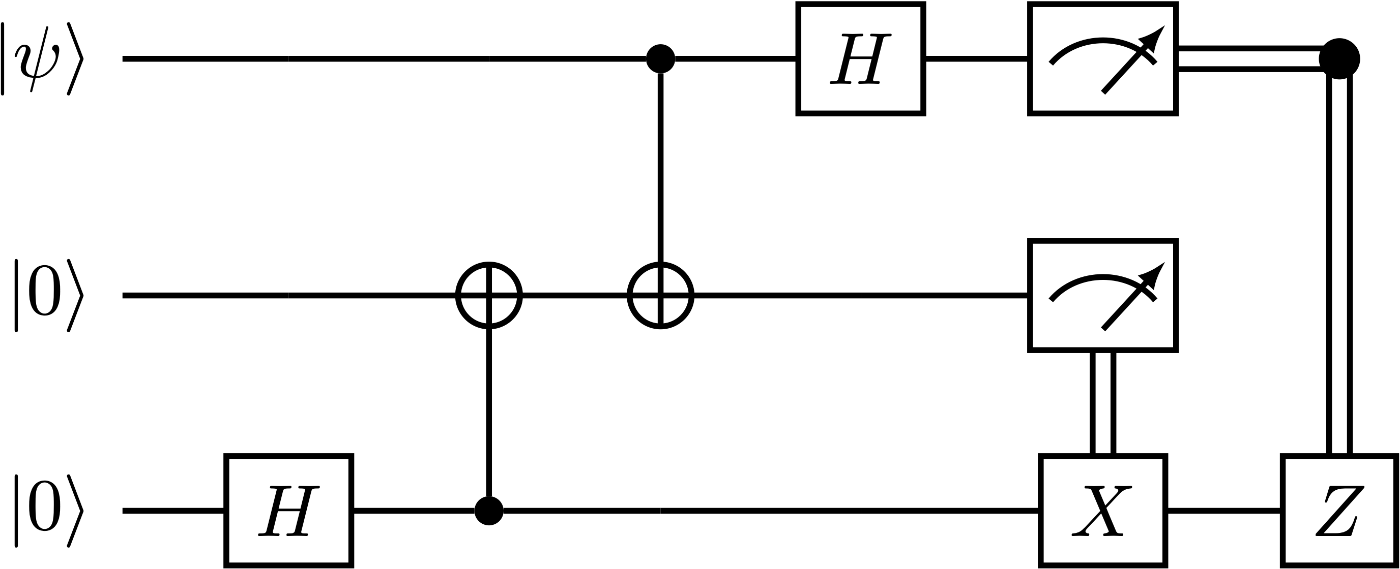

后选择

在 TensorCircuit 中通过 post_select 方法启用后选择。这允许用户通过 keep 参数选择量子位的 \(Z\) 测量后状态。 与 cond_measure 不同，post_select 返回的状态是折叠的，但不是归一化的。

c = tc.Circuit(2, inputs=np.array([1, 0, 0, 1] / np.sqrt(2)))
c.post_select(0, keep=1)  # 测量 qubit 0，对结果 1 进行后选择
c.state()

<tf.Tensor: shape=(4,), dtype=complex64, numpy=
array([0.        +0.j, 0.        +0.j, 0.        +0.j, 0.70710677+0.j],
      dtype=complex64)>

这个例子初始化了一个 \(2\)-qubit 最大纠缠态 \(\vert{\psi}\rangle = \frac{\vert{00}\rangle+\vert{11}\rangle}{\sqrt{2}}\)。 然后在 \(Z\)-basis 中测量第一个量子比特 (\(q_0\))，并后选择对应于测量结果 \(1\) 的非归一化状态 \(\vert{11}\rangle/\sqrt{2}\)。 这种具有非归一化状态的后选择方案速度很快，例如，可用于探索各种量子算法和非平凡的量子物理学，例如测量引起的纠缠相变。

普通测量

c = tc.Circuit(3)
c.H(0)
print(c.measure(0, with_prob=True))
print(c.measure(0, 1, with_prob=True))

(<tf.Tensor: shape=(1,), dtype=float32, numpy=array([1.], dtype=float32)>, <tf.Tensor: shape=(), dtype=float32, numpy=0.5>)
(<tf.Tensor: shape=(2,), dtype=float32, numpy=array([1., 0.], dtype=float32)>, <tf.Tensor: shape=(), dtype=float32, numpy=0.49999997>)

请注意，在测量后状态不会坍缩的意义上，普通测量 API 是虚拟的。

for _ in range(5):
    print(c.measure(0, with_prob=True))

(<tf.Tensor: shape=(1,), dtype=float32, numpy=array([0.], dtype=float32)>, <tf.Tensor: shape=(), dtype=float32, numpy=0.49999997>)
(<tf.Tensor: shape=(1,), dtype=float32, numpy=array([1.], dtype=float32)>, <tf.Tensor: shape=(), dtype=float32, numpy=0.5>)
(<tf.Tensor: shape=(1,), dtype=float32, numpy=array([0.], dtype=float32)>, <tf.Tensor: shape=(), dtype=float32, numpy=0.49999997>)
(<tf.Tensor: shape=(1,), dtype=float32, numpy=array([0.], dtype=float32)>, <tf.Tensor: shape=(), dtype=float32, numpy=0.49999997>)
(<tf.Tensor: shape=(1,), dtype=float32, numpy=array([0.], dtype=float32)>, <tf.Tensor: shape=(), dtype=float32, numpy=0.49999997>)

让我们即时编译 measure！（仔细的随机数操作）。

n = 3
key = K.get_random_state(42)


def measure_on(param, index, key):
    K.set_random_state(key)
    c = tc.Circuit(n)
    for i in range(n):
        c.rx(i, theta=param[i])
    return c.measure(*index)[0]


measure_on_jit = K.jit(measure_on, static_argnums=1)

key1 = key
for _ in range(30):
    key1, key2 = K.random_split(key1)
    print(measure_on_jit(K.ones([n]), [0, 1, 2], key2))

tf.Tensor([0. 0. 0.], shape=(3,), dtype=float32)
tf.Tensor([0. 1. 0.], shape=(3,), dtype=float32)
tf.Tensor([0. 1. 0.], shape=(3,), dtype=float32)
tf.Tensor([0. 0. 0.], shape=(3,), dtype=float32)
tf.Tensor([0. 1. 0.], shape=(3,), dtype=float32)
tf.Tensor([0. 0. 0.], shape=(3,), dtype=float32)
tf.Tensor([0. 0. 0.], shape=(3,), dtype=float32)
tf.Tensor([0. 0. 0.], shape=(3,), dtype=float32)
tf.Tensor([0. 0. 0.], shape=(3,), dtype=float32)
tf.Tensor([0. 0. 0.], shape=(3,), dtype=float32)
tf.Tensor([0. 0. 0.], shape=(3,), dtype=float32)
tf.Tensor([0. 0. 0.], shape=(3,), dtype=float32)
tf.Tensor([0. 1. 0.], shape=(3,), dtype=float32)
tf.Tensor([0. 0. 0.], shape=(3,), dtype=float32)
tf.Tensor([0. 1. 0.], shape=(3,), dtype=float32)
tf.Tensor([0. 0. 1.], shape=(3,), dtype=float32)
tf.Tensor([1. 0. 0.], shape=(3,), dtype=float32)
tf.Tensor([0. 0. 0.], shape=(3,), dtype=float32)
tf.Tensor([0. 0. 0.], shape=(3,), dtype=float32)
tf.Tensor([1. 1. 0.], shape=(3,), dtype=float32)
tf.Tensor([0. 0. 1.], shape=(3,), dtype=float32)
tf.Tensor([0. 0. 0.], shape=(3,), dtype=float32)
tf.Tensor([0. 0. 0.], shape=(3,), dtype=float32)
tf.Tensor([0. 1. 0.], shape=(3,), dtype=float32)
tf.Tensor([0. 0. 0.], shape=(3,), dtype=float32)
tf.Tensor([1. 0. 1.], shape=(3,), dtype=float32)
tf.Tensor([0. 0. 0.], shape=(3,), dtype=float32)
tf.Tensor([0. 0. 0.], shape=(3,), dtype=float32)
tf.Tensor([0. 0. 0.], shape=(3,), dtype=float32)
tf.Tensor([0. 1. 0.], shape=(3,), dtype=float32)

有关普通 measure 和我们在这里提到的两种测量类型之间差异的摘要，请参阅FAQ 文档.